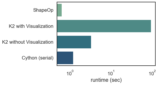
Performance Comparison Across Three Languages
ETA: The developer of Kangaroo2 (the C# implementation I've noted below) has informed me that his solver differs from ShapeOp in several key ways (so it's more of the same family of algorithms rather than a direct implementation of ShapeOp in another programming language). In his profiling, the assembly step that I hypothesized below as impacting the runtime is indeed responsible for the majority of the runtime of the solver component. The "solve" is on the order of <1 second without interruption for visual feedback, similar to ShapeOp. Additionally, ShapeOp did run to convergence in this case for this problem in 2000 iterations. YMMV in any profiling situation with only one sample problem, and my computer is slow!
I've fallen behind on blogging due to wrapping up some work responsibilities and finishing out my CA PE requirements before moving on with my career. Over the Christmas holidays, I got into working with Blender for structural analysis and formfinding visualization.
Why Blender? I've wanted for a long time to work more in open source software and buck the Rhino/Grasshopper ecosystem. I'm not a huge fan of visual programming either, so the opportunity to design my own interface without having to build buttons from scratch is a happy medium for me. Honestly, I've been blown away by some of the Blender generated simulations I've seen on Reddit, and I've wanted to implement the parallel dynamic relaxation solver that ShapeOp and Kangaroo2 use for some time.
I don't want to get into an argument about the semantics of whether these implementations are dynamic relaxation. Dynamic relaxation has been around since the 1960s, and it is still widely used today for structural formfinding, especially for long span gridshells like The British Museum Great Court.

From what I've seen, ShapeOp and Kangaroo2 have the same constraint formulation (i.e. the same relationship and derived "force vectors" between particles for structural element types: cables, bars, beams, shells) as dynamic relaxation. The methods differ in how (and how quickly!) they get from that initial position to the equilibrium position. The main appeal of ShapeOp/K2 vs. other implementations of dynamic relaxation is that it is stable and utilizes parallelism where it can to speed up the iterative process.
I first started working on my own implementation of this algorithm in Cython as part of a presentation I gave at PyGotham in the fall. To even come anywhere near the speed of the original C++ implementation (ShapeOp) or derived C# implementation (Kangaroo2), I needed to figure out how to achieve the parallelism of the algorithm in Python, which meant utilizing Cython to release the GIL.
While I was successful in achieving a 100x speedup over a pure Python implementation with a lot of list comprehensions, I'm still working through some kinks with Cython to see just how fast I can make it and address some lingering questions about parallelism with Cython. I've also wanted to see just how taxing it is to provide visual feedback during a simulation. As such, I've done a few tests with ShapeOp, Kangaroo2, and my own implementation.
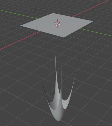
Once I started working in Blender, it was easy to set up a more complex test problem using its mesh library, but I still had to write parsers for ShapeOp and Cython to get out of blender based geometry. I took a flat plane and applied anchors to the four corners, then set up a 50x50 grid discretization resulting in 2500 points, and created dummy cables out of the mesh edges before applying a uniform load to all of the points. I wanted to apply an extreme deformation from the initial surface just to have some contrast in how quickly the algorithm convergences (the initial moves are quite large, but the final ~10% to the final position takes ~50% of the iterations).
ShapeOp Implementation
I would classify the original ShapeOp implementation as academic abandonware. The source code has a few 'fix this' comments that will never be sorted out, since the last time the website was updated was in 2016. The best technical but non jargony explanation for the algorithm itself is contained in the PhD thesis of Mario Deuss, though there are a few other papers that are either more jargony or less technical depending on the audience. There is a Python wrapper implemented from SWIG, but it is woefully incomplete. There is no way to set convergence criteria to tell the simulation to end; you can only set a maximum iteration number. For the global solve step, ShapeOp offers several different solvers in C++ (Simplicial LDLT, CG, MINRES, SOR), but it's not possible to set which one you want to use from the SWIG generated Python API, which defaults to Simplicial LDLT. For the test problem, I can't do a comparison based on accuracy (whether ShapeOp gets to the equilibrium position in fewer iterations), but I can do a comparison based on how long it takes ShapeOp for the same number of iterations as the C# implementation in Kangaroo2. ShapeOp took 0.63 seconds to run 2000 iterations, and I compiled ShapeOp with openMP enabled. (ETA: ShapeOp does have an interface in Grasshopper, same as Kangaroo2 below, but it hasn't been fully developed).
Kangaroo2 Implementation
A good chunk of the code for the Kangaroo2 implementation is hosted on Github, but this only provides the "local" solve step of the ShapeOp algorithm. The local assembly functions and global solve steps are unavailable, but if I had to hazard a guess, it utilizes Parallel.for loop for the local solve, which is easy to implement in C# (if only it were so easy in Python!). Interestingly, testing out the different solvers in Grasshopper shows just how much slower it is to visualize the intermediate steps to convergence, as the "Zombie" solver takes ~3 seconds to converge (Zombie meaning there is no visual feedback during the simulation), while the normal solver takes a little over a minute and a half to converge (updating the visualization in Rhino every 10 steps). I'm not sure how much overhead there is in the profiling widget in Grasshopper, so it's possible that these numbers are a bit conservative. I also can't separate out the assembly step (everything other than the actual iterative portion), so that would also ding the performance slightly.
Cython Implementation
Similar to Kangaroo2, I have convergence criteria in my implementation, so when movements between steps are small enough (we're talking order of fractions of millimeters), the simulation ends. Compared to Kangaroo2, I get a similar number of iterations for the same problem and similar convergence criteria, but again, I can't do an apples to apples comparison since that part of the program is closed source. I'm still struggling with the parallelization in Cython, as I think I need to be more explicit about thread allocation. The 2500 point problem runs, but the position values shoot off to infinity and NaN. However, even with the serial implementation in Cython, I'm getting a runtime of 1.5 seconds in the solver (no visualization included) for 2170 iterations. Interestingly, using cProfile has an enormous impact on the runtime, with an average 5 seconds per run, vs. 1.5 seconds using the time module. Most of the lag time in Blender as shown above is due to using list comprehensions to load the mesh into Cython from Blender (about 4 seconds out of the 5.5 profiled), so there's definite room for improvement. I also found profilehooks really useful for quickly getting profiled functions in the blender interface.